This analysis study explains by example how Vampir can be used to discover performance problems in your code and how to correct them.
Introduction
In many cases the Vampir suite has been successfully applied to identify performance bottlenecks and assist their correction. This article illustrates one optimization process to show in which ways the provided toolset can be used to find performance problems in program code. The following example demonstrates a three-part optimization of a weather forecast model with added simulation of cloud microphysics. Every run of the code has been performed on 100 cores with manual function instrumentation, MPI communication instrumentation, and recording of the number of L2 cache misses.

Figure 1 - Master Timeline (left) and Function Summary (right) showing an initial and unoptimized run of the weather forecast simulation
Getting a grasp of the program's overall behavior is a reasonable first step. The Vampir GUI in Figure 1 provides a high-level overview of the model's code execution. The Master Timeline chart at the left shows all 100 processes, with different colors representing the execution of specific functions over time. The Function Summary chart at the right provides statistics about these functions. For easier analysis, Vampir can sort related functions into specific groups. For this application the groups are: MPI - all functions belonging to MPI, METEO - functions computing the weather model, MP and MP_UTIL - functions computing the cloud microphysics, COUPLE - code coupling weather model with cloud microphysics, VT_API - functions related to the measurement system, Application - all remaining functions not fitting in any other group, e.g., main.
One run of the instrumented program took about 290 seconds to finish. In its first half (Section A in Figure 1), the program performs initialization tasks. Processes get started and synced, input is read and distributed among these processes. The preparation of the cloud microphysics (function group: MP) is done here as well.
The second half is the iteration part (Section B in Figure 1), where the actual weather forecasting takes place. In a normal weather simulation this part would be much larger. But in order to keep the recorded trace data and the overhead introduced by tracing as small as possible, only a few iterations have been recorded. This is sufficient as iterations are all doing approximately the same work in this program. Therefore, the simulation has been configured to only forecast the weather 20 seconds into the future. The iteration part consists of two major iterations (Sections B and C in Figure 1), each calculating 10 seconds of forecast. Each of these in turn is partitioned into several smaller inner iterations.
For our observations we focus only on two of these small, inner iterations, since this is the part of the program where most of the time is spent. The initialization work does not increase with a higher forecast duration and would only take a relatively small amount of time in a realistic run. The constant part at the beginning of each major iteration takes less than a tenth of the whole iteration time. Therefore, by far the most time is spent in the inner iterations. Thus, they are the most promising candidates for optimization.
All following screenshots are in a before-and-after fashion to point out what changed by applying the specific optimizations.
Identified Problems and Solutions
Computational Imbalance
A varying size of work packages (thus varying processing time of this work) means waiting time in subsequent synchronization routines. This section points out two easy ways to recognize this problem.
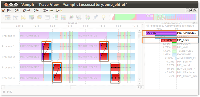
Figure 2 - Before Tuning: Master Timeline and Function Summary identifying MICROPHYSICS (purple color) as predominant and unbalanced
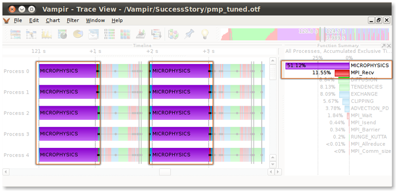
Figure 3 - After Tuning: Master Timeline and Function Summary showing a balanced computation along with an improvement in communication behavior
Problem
As shown in Figure 2, each occurrence of the MICROPHYSICS-routine (purple color) starts at the same time on all processes inside one iteration but takes between 1.3 and 1.7 seconds to finish. This imbalance leads to idle time in subsequent synchronization calls on the processes 1 to 4, because they have to wait for process 0 to finish its work (marked parts in the top figure). This is wasted time which could be used for computational work if all MICROPHYSICS-calls would have the same duration. Another hint at this overhead in synchronization is the fact that the MPI receive routine spends 17.6% of the time of one iteration as shown in the Function Summary chart at the right side in Figure 2.
Solution
To even out this asymmetry, the code which determines the size of the work packages for each process had to be changed. To achieve the desired effect, an improved version of the domain decomposition has been implemented. Figure 3 shows that all occurrences of the MICROPHYSICS-routine are vertically aligned, thus balanced. Additionally, the MPI receive routine calls are now visibly smaller than before. Comparing the Function Summary charts between both figures shows that the relative time spent in MPI receive has been decreased, and in turn the time spent inside MICROPHYSICS has been increased greatly. This means that the program now spends more time computing and less time communicating, which is the goal of this optimization.
Serial Optimization
Inlining of frequently called functions and elimination of invariant calculations inside loops are two ways to improve serial performance, namely code within a single MPI process. This section shows how to detect candidate functions for serial optimization and suggests measures to speed them up.
Problem
All performance charts in Vampir present information according to the user-selected time span in the timeline. Thus, the most time-intensive routine of one iteration can be determined by directly zooming into one or more iterations and analyzing the Function Summary chart. The function with the largest bar/value takes up the most time. In this example - Figure 2 - the MICROPHYSICS-routine can be identified as the most costly part of an iteration. Therefore, it is a promising candidate for gaining speedup through serial optimization techniques.
Solution
To get a fine-grained view of the MICROPHYSICS-routine's inner workings, it was required to trace the program using full function instrumentation. Only then it was possible to inspect and measure subroutines of MICROPHYSICS. This way, the most time-consuming subroutines have been identified and could be analyzed for potential optimization.
The review showed that a couple of small functions where called very often. Inlining such functions can improve performance greatly. Using the metric Number of invocations in the Function Summary chart allows to analyze how often a function is called.
The second inefficiency the analysis revealed had been invariant calculations performed inside loops. Such calculation can be moved before the respective loops to improve performance.
Figure 3 sums up the tuning of the computational imbalance and the serial optimization. The timeline shows that the duration of the MICROPHYSICS-routine is now equal among all processes. Through serial optimization its duration has been decreased from about 1.5 seconds to 1.0 second. This decrease in duration of about 33% is a good result given the simplicity of the performed changes.
High Cache Miss Rate
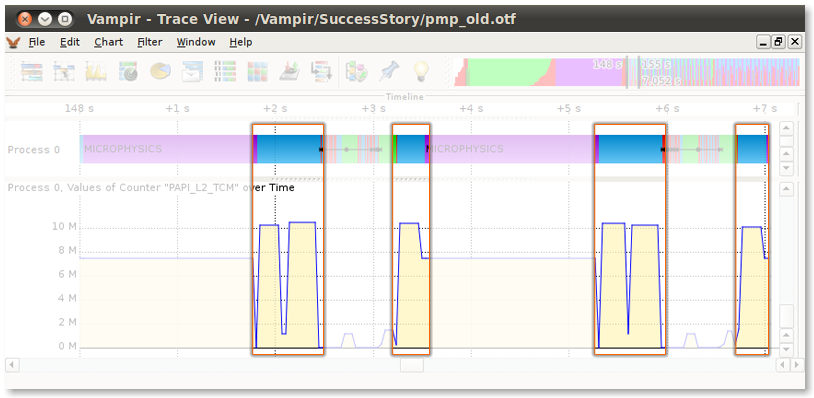
Figure 4 - Before Tuning: Counter Data Timeline revealing a high amount of L2 cache misses inside the CLIPPING-routine (light blue)
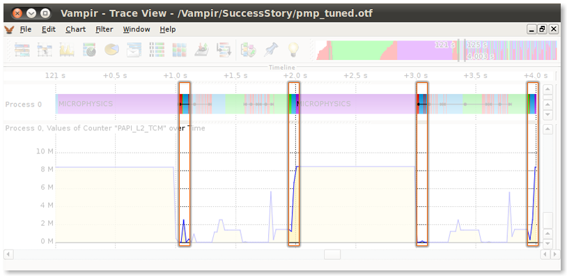
Figure 5 - After Tuning: Clearly visible improvement of cache usage and reduced execution time
The latency gap between cache and main memory is about a factor of 8. Therefore, optimizing for cache usage is crucial for performance. If data is not accessed in a linear fashion as the cache expects, cache misses occur and the specific instructions have to suspend execution until the requested data arrives from main memory. A high cache miss rate therefore indicates that performance might be improved through reordering of the memory access pattern to match the cache layout of the platform.
Problem
As shown in the Counter Data Timeline - bottom chart in Figure 4 - the CLIPPING-routine (light blue) causes a high amount of L2 cache misses. Also, its long duration alone is sufficient to make it a candidate for inspection. What caused these inefficiencies in cache usage were nested loops, which accessed data in a very random, non-linear fashion. Data access can only profit from cache if subsequent read calls access data in the vicinity of previously accessed data.
Solution
Reordering of the nested loops to match the memory order improved the cache behavior. The tuned version of the CLIPPING-routine now needs only a fraction of the original time as shown in Figure 5.
Conclusion
The analysis of the weather forecast program revealed three performance issues. By addressing each issue and optimizing the inefficient parts of the code, the duration of one iteration could be reduced from 3.5 seconds to 2.0 seconds.
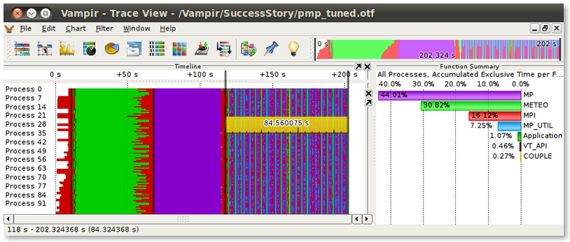
Figure 6 - Overview of the optimized weather forecast simulation showing significantly improved performance
As indicated by the ruler in Figure 6, the two major iterations now take about 85 seconds to finish. Whereas in the unoptimized version shown in Figure 1, they required about 140 seconds, resulting in a total speed gain of 40%.
The detailed insight into the program's runtime behavior, provided by the Vampir toolkit, enabled this significant performance improvement.
-- Matthias Weber (Technical University Dresden and Vampir)