Profiling tools such as HPCToolkit, Caliper, TAU, and Score-P allow developers to focus their optimization efforts by pinpointing the parts within a code's execution that consume the most time. Most profiling tools use their own unique format to store recorded data, and they may display this data as text or with a tool-specific viewer (typically a GUI). The analysis capabilities in these tools are limited in the kinds of analyses they support, and they do not enable the end user to programmatically analyze performance data.
Hatchet is a Python-based library that allows performance profiles to be stored as Pandas DataFrames, indexed by structured tree and graph data. It is intended for analyzing performance data that has a hierarchy (for example, serial or parallel profiles that represent calling context trees, call graphs, nested regions’ timers, etc.). Hatchet implements various operations to analyze a single hierarchical dataset or compare multiple datasets, and its API facilitates analyzing such data programmatically.
Usage
Hatchet supports analyzing data from several profiling tools: HPCToolkit, Caliper, gprof, callgrind, and Python’s cprofile. We are in the process of adding support for TAU, and we welcome contributions that add support for other profiling tools/data formats. Step zero for using Hatchet is collecting data for a program with the tool of one’s choice (see supported data formats.) Once the user has a dataset to analyze, they can install Hatchet either using pip or directly cloning the git repository on GitHub. Hatchet can then be used in a jupyter notebook or an interactive Python session, using:
>>> import hatchet as ht
After importing hatchet, a user can load their profile data into Hatchet using the corresponding reader. Once the data is loaded in Hatchet, it will be stored into Hatchet’s data structure known as GraphFrame. The GraphFrame contains two objects: 1. a graph object that stores the caller-callee relationships, and 2. a Pandas DataFrame that stores the categorical or numerical data for each node in the graph. This is shown in Figure 1.
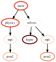
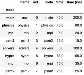
Figure 1: Hatchet’s central data structure is known as a GraphFrame. The GraphFrame consists of two components, a graph storing the caller-callee relationships and a pandas DataFrame object containing the data associated with each node in the graph.
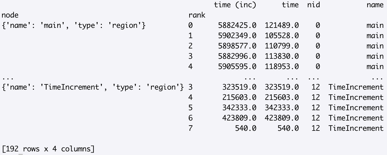
The hatchet API has several operations that users can perform on a single graphframe (dataset) or on multiple graphframes. For example, after loading a dataset into a GraphFrame, a user can visualize the graph in the terminal and print the corresponding DataFrame using the Python code below. For this example, we assume the GraphFrame created by the user has been named gf:
>>> print(gf.tree())

>>> gf.dataframe
We also support other visualization formats described here. Once the user is familiar with the GraphFrame data structure and what it contains, they can use various Hatchet operations to analyze their hierarchical data or graph. For example, a user can prune the tree to focus on an interesting part of the graph using the filter and squash operations. Hatchet provides the option to filter on the metrics stored in the DataFrame or on callpath patterns in the graph or both. Hatchet provides a query language that can be used to construct a query that specifies a callpath pattern that can be provided as an argument to filter.
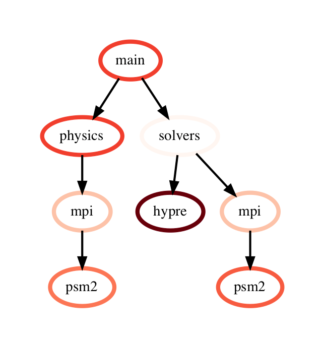
A user can also load two datasets into separate GraphFrames, and use Hatchet’s algebraic operators (add, subtract, divide, or multiply) to compare them. Some common use cases are comparing execution profiles that represent two executions of a program that differ in some aspect -- runs with different inputs, or runs with different number of MPI processes or threads, or simply executions done at different points in time. For example, to understand the differences in time spent in different nodes of call graphs from two executions, a user can simply write:
>>> gf3 = gf2 - gf1
This performs a pairwise difference of the numeric metrics associated with corresponding nodes in the two graphs, creating nodes as needed when a node only exists in one of the graphframes which is shown in Figure 2.
 -
- 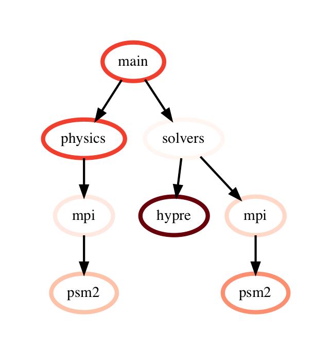 =
= 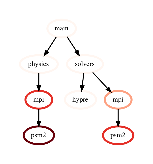
Figure 2: Subtraction operation on two GraphFrames (resulting graph on the right). The color of node represents the exclusive time spent in the node on a linear color scale.
With a few lines of Python code, a user can also compare several performance profiles as shown here. We refer the reader to the hatchet documentation for the complete Hatchet API and usage examples.
Summary
Hatchet is a Python-based performance analysis tool for pinpointing bottlenecks in hierarchical or structured data, such as calling context trees or call graphs. By performing simple operations on these graphs with Hatchet, users can get answers to questions such as:
- Which functions in my code have the most load imbalance?
- Which functions or code blocks scale poorly?
- Which functions speed up the most when using CPUs versus GPUs?
To get started with Hatchet, we refer the reader to the links below:
-- Abhinav Bhatele (University of Maryland), Stephanie Brink (Lawrence Livermore National Laboratory)
Contact: hatchet-help@listserv.umd.edu