Attempting to optimise performance of a parallel code can be a daunting task, and often it is difficult to know where to start. To help address this issue, the POP methodology supports quantitative performance analysis of parallel codes to measure the relative impact of the different factors inherent in parallelisation. A feature of the methodology is that it uses a hierarchy of metrics, each metric reflecting a common cause of inefficiency in parallel programs. These metrics then allow comparison of parallel performance (e.g. over a range of thread/process counts, across different machines, or at different stages of optimisation and tuning) to identify which characteristics of the code contribute to inefficiency. This article introduces these metrics, explains their meaning, and provides insight into the thinking behind them.
Acquiring performance data
The first step to calculating these metrics is to use a suitable tool (e.g. Extrae or Score-P) to generate trace data whilst the code is executed. The traces contain information about the state of the code at a particular time (e.g. it is in a communication routine or doing useful computation) and also contains values from processor hardware counters (e.g. number of instructions executed, number of cycles).
The metrics are then calculated as efficiencies between 0 and 1, with higher numbers being better. However, in some cases, this value can be greater than 1. In general, we regard efficiencies above 0.8 as acceptable, whereas lower values indicate performance issues that need to be explored in detail. When you work with POP, the data from your application will be collected and, basing on that, the corresponding metrics computed. The results then will be presented in the form of Parallel Application Performance Assessment, which includes a root cause analysis of the performance issues that were identified. The ultimate goal then for POP is rectifying these underlying issues, e.g. by the user, or as part of a POP Proof-of-Concept follow-up activity.
In general, the POP methodology is applicable to various parallelism paradigms, however for simplicity the POP metrics presented here are discussed in the context of distributed-memory message-passing with MPI and shared-memory threading with OpenMP. For this, the following values are calculated for each process and/or thread from the trace data: time doing useful computation, time spent for communication or synchronization inside the parallel runtime system (MPI/OpenMP), number of instructions & cycles during useful computation. Useful computation excludes time within the overheads of parallelism. The following sections will first present the MPI-centric initial POP metrics and then the two extensions to support hybrid parallel programs with a focus on MPI + OpenMP.
Hierarchy of metrics
At the top of the hierarchy is Global Efficiency (GE), which we use to judge overall quality of parallelisation. Typically, inefficiencies in parallel code have two main sources:
-
Overheads imposed by the parallel execution of a code, i.e., the parallel programming model and its corresponding runtime
-
Poor scaling of computation with increasing numbers of processes and/or threads
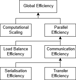
Fig. 1 POP Standard Metrics for Parallel Performance Analysis
To quantify this, we define two sub-metrics to measure these two inefficiencies. These are Parallel Efficiency and Computational Scaling, and our top-level GE metric is the product of these two sub-metrics:
GE = Parallel Efficiency * Computational Scaling
Parallel Efficiency (PE) reveals the inefficiency in splitting computation over processes and then communicating data between processes. As with GE, PE is a compound metric whose components reflect two important factors in achieving good parallel performance in code:
-
Ensuring even distribution of computational work across processes
-
Minimising time communicating data between processes
These are computed with Load Balance Efficiency and Communication Efficiency, and PE is defined as the product of these two sub-metrics:
PE = Load Balance * Communication Efficiency
At the same time PE is computed as the ratio between average useful computation time (across all processes) and total runtime:
PE = average useful computation time / total runtime
Load Balance (LB) is computed as the ratio between average useful computation time (across all processes) and maximum useful computation time (also across all processes):
LB = average useful computation time / maximum computation time
Communication Efficiency (CommE) is the maximum across all processes of the ratio between useful computation time and total runtime:
CommE = maximum computation time / total runtime
CommE identifies when code is inefficient because it spends a large amount of time communicating rather than performing useful computations. CommE is composed of two additional metrics that reflect two causes of excessive time within communication:
-
Processes waiting at communication points due to the temporal imbalance (i.e. serialisation).
-
Processes transferring large amounts of data relative to the network capacity (limited to the network transfer speed) or with high-frequent communication (limited by the network latency).
These are computed using Serialisation Efficiency and Transfer Efficiency. In obtaining these two sub-metrics we first calculate (using the Dimemas simulator) how the code would behave if executed on an idealised network where transmission of data takes zero time.
Serialisation Efficiency (SerE) describes any loss of efficiency due to dependencies between processes causing alternating processes to wait:
SerE = maximum computation time on ideal network / total runtime on ideal network
Transfer Efficiency (TE) represents inefficiencies due to time in data transfer:
TE = total runtime on ideal network / total runtime on real network
These two sub-metrics combine to give Communication Efficiency:
CommE = Serialisation Efficiency * Transfer Efficiency
The final metric in the hierarchy is Computational Scaling (CompS), which are ratios of total time in useful computation summed over all processes. For strong scaling (i.e. problem size is constant) it is the ratio of total time in useful computation for a reference case (e.g. on 1 process or 1 compute node) to the total time as the number of processes (or nodes) is increased. For CompS to have a value of 1 this time must remain constant regardless of the number of processes.
Insight into possible causes of poor computation scaling can be investigated using metrics devised from processor hardware counter data. Two causes of poor computational scaling are:
-
Dividing work over additional processes increases the total computation required
-
Using additional processes leads to contention for shared resources
-
Hardware might run at different frequency for subsequent runs
and we investigate these using Instruction Scaling, Instructions Per Cycle (IPC) Scaling, and Frequency Scaling.
Instruction Scaling is the ratio of total number of useful instructions for a reference case (e.g. 1 processor) compared to values when increasing the numbers of processes. A decrease in Instruction Efficiency corresponds to an increase in the total number of instructions required to solve a computational problem.
IPC Scaling compares IPC to the reference, where higher values indicate that rate of computation has increased. Typical causes for this include increasing cache hit rate, as a result of smaller partition of work in strong scaling.
In addition to that, Frequency Scaling compares the average frequency during useful computation to the architecture’s reference. This metric indicates changes in the dynamic frequency selection of the hardware and can explain runtime variation for execution with same parameters and efficiencies. It is also a relevant factor in the analysis of scaling within one node, as increasing the number of cores being used typically implies a reduction in the processor frequency.
Support for hybrid parallelism
Hybrid Parallelism combines multiple parallel programming paradigms in a single program to harness the full power of modern HPC systems, e.g. MPI and OpenMP. There are two extension to support hybrid parallel programs with the POP methodology: the additive and the multiplicative metrics. The different approaches leave the Parallel Efficiency (PE) as introduced above the same, but the sub metrics are different.
All metrics in the additive model are defined relatively to the runtime. This model can alternatively be defined using inefficiency metrics, where each inefficiency value is defined as 1 minus the corresponding efficiency. It is described as additive because child inefficiency values can be summed to give a parent inefficiency.
In contrast to that, in the multiplicative model the product of the child metrics creates a parent metric.
The additive efficiency metrics measure absolute cost of each performance bottleneck, using a set of metrics that are based on concepts specific to each programming model. This makes it easy to map the metrics values to concepts and issues easily understandable by the software engineer. In contrast, the multiplicative metrics closely extends the MPI approach keeping an abstract and generic classification of the classifying all bottlenecks as either load balance, communication, irrespective of the programming paradigm. In the hybrid model, any source of inefficiency that is not caused by any corresponding MPI inefficiency, is caused by the other level of parallelism.
Additive hybrid model
The additive approach considers processes (MPI) and threads (OpenMP) separately and splits the Parallel Efficiency into Process Efficiency and Thread Efficiency:
Parallel Efficiency = Process Efficiency + Thread Efficiency – 1
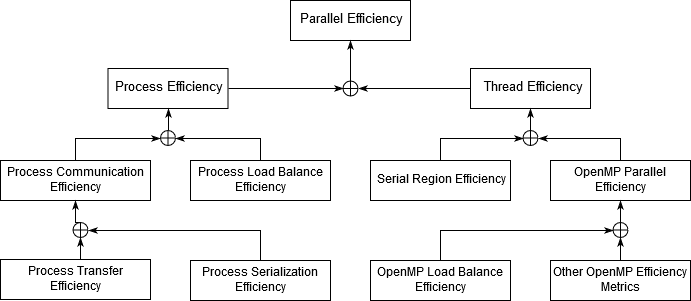
Fig. 2 Additive Hybrid Model
Process Efficiency measures inefficiences due to the MPI message-passing parallelization when ignoring the threads. For process efficiency time in useful computation outside OpenMP, and time in OpenMP, are both considered as useful time. Hence time in MPI outside OpenMP is considered non-useful.
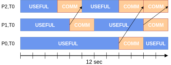
The concepts of Communication Efficiency, Load Balance Efficiency, Transfer Efficiency and Serialization Efficiency have been introduced above. The following examples review and illustrate these concepts:
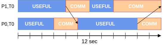 P1,T0: Computation: 6 sec, Communication: 6 sec.
P0,T0: Computation: 8 sec, Communication: 4 sec.
The Process Efficiency is computed as the average useful time divided by the runtime: 7 / 12 = 58.3 %.
The Process Communication Efficiency is computed as the maximum useful time divided by the runtime: 8 / 12 = 66.7 %.
The Process Load Balance Efficiency is computed as runtime minus the difference of the maximum and the average useful time, all divided by the runtime: 91.7 %.
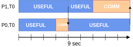
The Process Transfer Efficiency is computed as the program’s simulated runtime on an ideal network divided by the program’s runtime on a real network: 9 / 12 = 75.0%.
The Process Serialization Efficiency is computed as one minus the difference of the Process Transfer Efficiency and the Process Communication Efficiency: 1-(0.75-0.667) = 91,7%.
Thread Efficiency measures the cost of inefficient thread parallelisation. Therefore, it is computed as the runtime minus average of the useful serial computation (per process) minus the average time within OpenMP regions (per process) plus average useful computation (per thread), all divided by the runtime.
The Thread Efficiency can be split up into the Serial Region Efficiency and the OpenMP Parallel Region Efficiency. The serial efficiency follows the concept of Amdahl’s law by relating the average serial useful computation time to the number of threads per process.
Thread Efficiency = OpenMP Parallel Efficiency + Serial Region Efficiency – 1
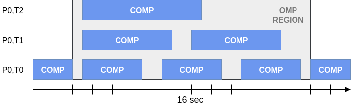 P0,T2: OMP Computation: 1 x 6 sec.
P0,T1: OMP Computation: 2 x 4.5 sec.
P0,T0: OMP Computation: 3 x 3 sec.
In this example, the OpenMP Parallel Region Efficiency is 1 – (12 - 8) / 16 = 75% and the Serial Region Efficiency is 1 – (4x2 / 3) / 16 = 83 %.
Multiplicative hybrid model
The multiplicative approach decomposes the hybrid parallel programs’ efficiency as follows:
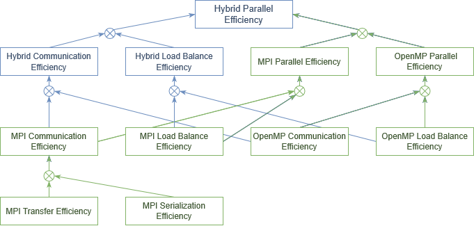
Fig. 3 Multiplicative hybrid model
The Hybrid Parallel Efficiency is equivalent to the Parallel Efficiency of the additive model and meassures the percentage of time outside the two parallel runtimes. As in the original MPI model, this efficiency can be split between two components: global load balance and communication efficiencies.
The Hybrid Communication Efficiency reflects the loss of efficiency by hybrid communication and is split into the MPI and the OpenMP contributions. It is computed as the maximum useful computation time (over all processes, threads) divided by the program’s runtime. Here, the useful computation time excludes time spent both the MPI and OpenMP runtimes.
The Hybrid Load Balance Efficiency reflects how well the distribution of work to processes or threads is done in the hybrid application and is split into the MPI and the OpenMP contributions. It is computed as the average useful computation time (over all processes, threads) divided by the maximum useful computation time (over all processes, threads).
The MPI Parallel Efficiency describes the parallel execution of the code in MPI considering that from the MPI point of view, the OpenMP runtime is as useful as the computations. Similarly, to the original POP metrics model, can be computed by multiplying the MPI Load Balance and MPI Communication Efficiency metrics as follows:
MPI Parallel Efficiency = MPI Comm Efficiency x MPI Load Balance
The MPI Communication Efficiency describes the loss of efficiency in MPI processes communication, as described above in the second section, only considering time outside MPI.
The MPI Load Balance Efficiency describes the distribution of work in MPI processes as described above in the second section, only considering time outside MPI.
Regarding MPI, there are also the MPI Transfer Efficiency and MPI Serialization Efficiency, which describes loss of efficiency due to actual data transfer and data dependencies. The concept of both was described above.
 P2,T0: Computation 6 sec, Communication: 6 sec.
P1,T0: Computation 8 sec, Communication: 4 sec.
P0,T0: Computation 10 sec, Communication: 2 sec.
In this example, the MPI Parallel Efficiency is 8 / 12 = 66.6%, the MPI Load Balance is 8 / 10 = 80%, the MPI Communication Efficiency is 10 / 12 = 83.3 %, the MPI Transfer Efficiency is 10 / 12 = 83.3 %, and the MPI Serialization Efficiency is 100 %.
In the multiplicative model, any efficiency that is not assigned to the corresponding MPI efficiency, is caused by the other level of parallelism. In the combination of MPI and OpenMP, this is OpenMP, as described below.
This hybrid execution example extends above example by some OpenMP worker threads. The calculation of MPI metrics provides the same results.
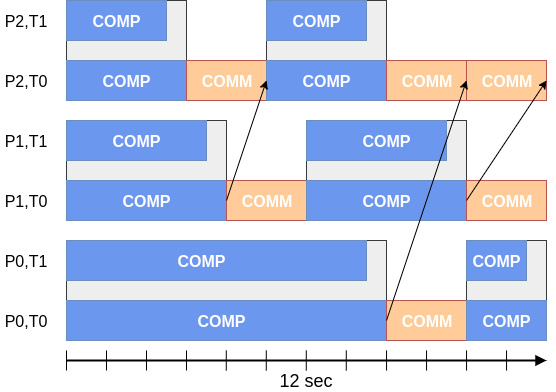 P2,T1: OMP Computation: 5 sec.
P2,T0: OMP Computation: 6 sec.
P1,T1: OMP Computation: 7 sec.
P1,T0: OMP Computation: 8 sec.
P0,T1: OMP Computation: 9 sec.
P0,T0: OMP Computation: 10 sec.
In this example, the Hybrid Parallel Efficiency is 7.5 / 12 = 62.5%, the Hybrid Load Balance is 7.5 / 10 = 75.0% , and the Hybrid Communication Efficiency is 10 / 12 = 83.3%.
The OpenMP Parallel Efficiency describes the parallel execution of the code in OpenMP and, similarly to the original POP metrics model, can be computed by multiplying the OpenMP Load Balance and OpenMP Communication Efficiency metrics as follows:
OpenMP Parallel Efficiency = OpenMP Comm Efficiency x OpenMP Load Balance
Since it focuses purely on OpenMP, it also equals the quotient of the Hybrid Parallel Efficiency and the MPI Parallel Efficiency, and similarly, the average useful compute time (per process, thread) divided by the average time outside MPI (per process). For above example it calculates as 62.5% / 66.6% = 93.8%.
The OpenMP Communication Efficiency is defined as the quotient of the Hybrid Communication Efficiency and the MPI Communication Efficiency and thereby captures the overhead induced by the OpenMP constructs, which represents threads synchronization and scheduling. It is computed as the maximum of useful compute time (over all processes, threads) divided by the maximum runtime outside of MPI (per process). For above example it calculates as 83.3% / 83.3% = 100%.
Finally, the OpenMP Load Balance is defined as the quotient of the Hybrid Load Balance Efficiency and the MPI Load Balance Efficiency and represents the load balance within the OpenMP part of the program. For above example it calculates as 75% / 80% = 93.8%.
With this approach, OpenMP child efficiencies may be bigger than 1 if OpenMP improves the MPI metrics at hybrid level.
Summary
We sincerely hope this methodology is useful to our users and others and will form part of the project's legacy. If you would like to know more about the POP metrics and the tools used to generate them please check out the rest of the Learning Material on our website, especially the document on POP Metrics for a more formal definition.